Introduction to the Quantum Inspire API¶

Step 0: Create account and run a job via the web interface (demo in browser)¶

Step 1: SDK installation¶

Instead of the web interface, we can run advanced algorithms by interacting with the Quantum Inspire platform directly from python.
We assume that you already have a working python environment setup. If not, a possible way to create one using conda is by running

conda create --name EQTC_workshop python=3.8
conda activate EQTC_workshop

We first need to install the SDK. It's code is available on Github and is simply installable via pip:

pip install quantuminspire

For our next example, we will also need the following packages:

pip install numpy scipy matplotlib networkx qiskit

If you already have some of those packages installed, please make sure you are on the latest version (especially for qiskit).

Step 2: API authentication¶

Single-use authentication¶

We need to authenticate with the API by using the same account we created via the web interface.
We provide our credentials and pass them together with the URL to the API object. This is okay for a single use.

Alternative: token authentication¶

To avoid having to type our login information every time we start a new session, we can conveniently use the API token provided on the website account interface

My QI --> Account --> Your API Token

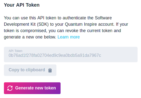
We only need to copy the token into the notebook and call save_account(), enable_account() once.
After that, only the call to get_authentication() is needed to retrieve the saved token and start a new session.
This allows to keep your token secret and not having to keep it in plain text in your code! (the token shown here is already invalidated)

Backends¶

In this example, we will first use the QX Emulator as backend. Then we will run our code on Starmon-5.
It is possible to ask the API for all available backends and their detailed information, like so:

This gives you important information, like the types of gates that are allowed on this backend and its topology (connectivity).
To choose a backend, we simply provide the result of the following call to the API object's execute_qasm() method (see below).

Deutsch–Jozsa algorithm description¶

In the Deutsch–Jozsa algorithm we use an oracle to determine if a binary function $$f(x) : \{0,1\}^n \rightarrow \{0,1\}$$ is constant or balanced.

A function is constant if $f(x)=0$ or $f(x)=1$ for all values of $x$.
A function is balanced if $f(x)=0$ for half of the possible input values $x$ and $f(x)=1$ for the other half.
The task is to distinguish the balanced case (half of all inputs yield output 1) from the constant case (all or none of the inputs yield output 1).
You can read more about this algorithm on Wikipedia or on the Quantum Algorithm Zoo.

What is it used for?¶

The Deutsch-Josza algorithm is a simple example of a quantum algorithm that can be used to speed up a search. As will be explained below, it can determine whether or not a function has a certain property (being balanced). The algorithm achieves this by requiring that the function (more precisely, a derivation of the function) need only be called once with a quantum algorithm instead of twice with a classical algorithm. When the function is very 'expensive', e.g., in terms of computational resources, it can be very beneficial if you have to compute this function only once instead of twice.

Although the speed-up of this specific case of a 2-to-1 bit function is only a factor of 2, in general this algorithm can achieve exponential speedup (for the worst case of the classical counterpart). Historically, this is the first well-defined quantum algorithm achieving a speedup over classical computation.

How does it work?¶

In this example we consider a binary function $f(x) : \{0,1\} \rightarrow \{0,1\}$. There are four possibilities for the function $f(x)$, which we call the Oracle function. These are:

1. $$f_1(x)=0$$
2. $$f_2(x)=1$$
3. $$f_3(x)=x$$
4. $$f_4(x)=1-x$$

The algorithm to determine whether our function $f(x)$ is constant or balanced requires only a single query of $f(x)$.

In this example, we will implement a very simple Oracle for the four different functions, but a much more complex Oracle could also be used.

Implementation in cQASM¶

The following code shows the implementation of the algorithm, which uses two qubits.

We use an oracle to determine if a binary function $f(x)$ is constant or balanced.
Here, the constant cases are $f(x)=fc1=0$ and $f(x)=fc2=1$, and balanced cases $f(x)=fb3=x$ and $f(x)=fb4=NOT(x)$.
By changing the Oracle, the 4 different functions can be tested.

Running a simulation¶

Let us generate a circuit for oracle $fc1$ and simulate it. What do you expect from the result?

You can find more information about executing an algorithm and examining results in the knowledge base.

We now call the execute_qasm method with our generate circuit-string and the desired simulation backend, and examine the histogram of results.

Not surprisingly, our perfect (noise-free) simulation of the quantum circuit gives a perfect result.
If we now run the same code again, but this time implement the 2nd Oracle, we would see that we get exactly the same result as for the first oracle.

Likewise, we can run the algorithm for Oracle 3 or Oracle 4. In these cases, we will get a different result:

Now let's try it on Starmon-5¶

Now things look very different! Due to the noise on a real quantum processor, we do not measure the correct result 100% of the time anymore.
However, we can still retrieve the correct answer with high probability, which is what usually matters in practice.

You have now learned how to connect to the Quantum Inspire API from a python session and execute cQASM-algorithms on different simulation- and hardware-backends.
Next, we will proceed with an example of QAOA, a more advanced algorithm that we can run on Quantum Inspire.